Spatial-temporal Checkouts
MAT 259, 2015
Donghao Ren
Concept
In this assignment, I built a visualization to show checkout trends of different kinds of books.
The idea is to use an algorithm to generate a 2D spatial layout for the books, and expand the 2D layout into a 3D volume with time.
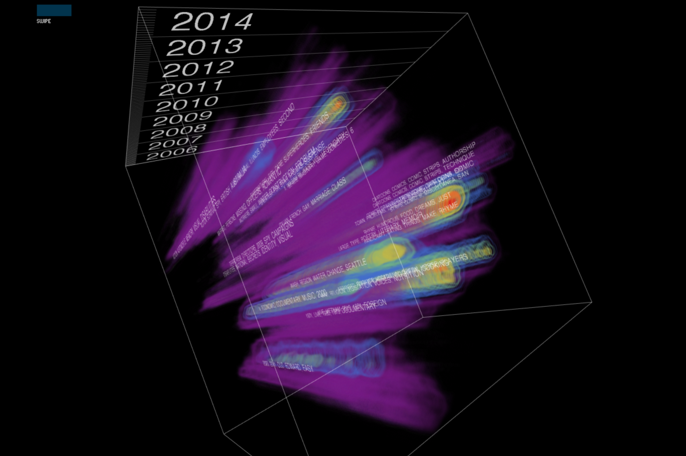
My design is a volumetric visualization, using the X-Y plane to layout the books, and the Z axis to show the checkout trend.
So each location (X, Y, Z) means the number of checkouts at book (X, Y) and time Z.
Query
There are multiple queries to build this visualization.
First we extract interesting keywords, those that occur most frequently.
SELECT keyword, occurrenceCount AS count
FROM x_keywordOccurrenceCount
ORDER BY count DESC LIMIT 1000
Then we get the keywords for each bib.
SELECT
  x_keyword.bibNumber AS bibNumber,
  GROUP_CONCAT(x_keyword.keyword) AS keywords
FROM
  x_keyword
WHERE
  keyword IN (%s)
GROUP BY bibNumber
Process
Book layout: The books are layout by their keywords. Similar books (with similar keywords) are placed closely in the layout.
The algorithm was a 2-layer RBM model. There are 807,493 books in the collection, each has a X, Y coordinate given by the algorithm.
The steps of the layout algorithm can be summarized as the following:
Rendering: Since volume rendering is not possible in Processing, I rendered the volume as 108 slices, corresponding to the 108 months from Jan. 2006 to Dec. 2014. The colors was chosen from a given gradient using shaders. So what you see in the picture is actually 108 transparent images stacked together, giving you a volumetric feeling.
The steps of the layout algorithm can be summarized as the following:
- Give the each keyword an index from 0 to N - 1
- For each bib, build a vector with N entries, the i-th entry is 1 if the bib has the i-th keyword, is 0 otherwise.
- Replicate the vectors for the bibs according to the checkouts, so that the bibs that are checkout more often appears more often.
- Use the vectors of the replicated bibs as the training examples of the RBM algorithm.
- Train the first layer RBM model.
- Train the second layer Gaussian RBM model with 2 hidden units, using the outputs of the first as input.
- Finally, from the output of the second layer, we have 2 variables, that can be used as the X, Y location for each book.
Rendering: Since volume rendering is not possible in Processing, I rendered the volume as 108 slices, corresponding to the 108 months from Jan. 2006 to Dec. 2014. The colors was chosen from a given gradient using shaders. So what you see in the picture is actually 108 transparent images stacked together, giving you a volumetric feeling.
Final result
Here's the final Processing-based visualization. There are multiple clusters in the layout, I extracted the clusters by a local-maximum finding algorithm, and then for each cluster, I generated a set of most important keywords using TF-IDF weighting. The important keywords for each cluster is rendered on the cluster.
From the visualization, we can see some clusters that only appeared a certain period of time, there is also some kind of temporal pattern for each year, such as the activity is lower during the Christmas weeks.
This image is a product of my AlloVolume project, rendered using a GPU-based ray casting algorithm. It also works in the Allosphere.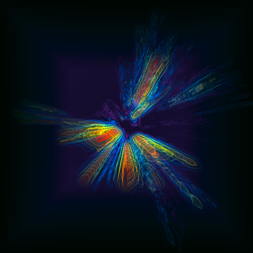
Code
I used Processing.
Source Code + Data
iPython scripts (very messy):
Keyword Extraction
RBM Adjustment
RBM Viewport
Bibpos Plot
Source Code + Data
iPython scripts (very messy):
Keyword Extraction
RBM Adjustment
RBM Viewport
Bibpos Plot