3D Visualisation of Spatially Situated Research in UCSB
MAT 259, 2018
Christina Last
Concept
As a researcher, how would you go about finding work similar to your own? Measures of similarity could include research done in similar regions of the world, research by similar departments and scholars, research with topical correspondence, or research that co-occurred at the same temporality, reflecting contextual change. Determining these measures of similarity from a digital text collection requires mining document metadata. This project experiments with mapping from non-spatial tabular meta-data to spatialisations.
Spatial information provides guidance for the ways in which people, places and topics can be meaningfully displayed and analysed. Spatialization embeds documents into a metaphorical space where documents in closer proximity can be perceived as similar. Different conceptualizations of similarity, such as geographic and topical, lend themselves to analysis through different spatializations with varying measures of distance. By spatializing information, researchers can compute on collections of research documents, asking questions like “Where in the world is the density of my domain’s research the highest?”, “Which domain is the most spatially diverse? or “What other research shares the same spatial neighborhood as my domain?”
Spatial information provides guidance for the ways in which people, places and topics can be meaningfully displayed and analysed. Spatialization embeds documents into a metaphorical space where documents in closer proximity can be perceived as similar. Different conceptualizations of similarity, such as geographic and topical, lend themselves to analysis through different spatializations with varying measures of distance. By spatializing information, researchers can compute on collections of research documents, asking questions like “Where in the world is the density of my domain’s research the highest?”, “Which domain is the most spatially diverse? or “What other research shares the same spatial neighborhood as my domain?”
Query
Query for Grouping research by Department
# summarize publication ids by department
# select all publications from departments with over 50 publications
"degree_gra" = 'University of California, Santa Barbara. Electrical and computer engineering' OR
"degree_gra" = 'University of California, Santa Barbara. Electrical and Computer Engineering' OR
"degree_gra" = 'University of California, Santa Barbara. Materials' OR
"degree_gra" = 'University of California, Santa Barbara. Chemistry' OR
"degree_gra" = 'University of California, Santa Barbara. Education' OR
"degree_gra" = 'University of California, Santa Barbara. Education - Gevirtz Graduate School' OR
"degree_gra" = 'University of California, Santa Barbara. Physics' OR
"degree_gra" = 'University of California, Santa Barbara. Computer Science' OR
"degree_gra" = 'University of California, Santa Barbara. Sociology' OR
"degree_gra" = 'University of California, Santa Barbara. Chemical Engineering' OR
"degree_gra" = 'University of California, Santa Barbara. History' OR
"degree_gra" = 'University of California, Santa Barbara. Psychology' OR
"degree_gra" = 'University of California, Santa Barbara. Geography' OR
"degree_gra" = 'University of California, Santa Barbara. Mechanical Engineering'
Query for Geoparsing Titles aand Abstracts of UCSB Research
import csv
import time
#import tab-delimited keywords file
f = open('gazetteers/us-places-clean.txt','r')
#gazetteer = f.read().lower().split("\r")
citylist = f.read().strip().split("\r")
f.close()
gazetteer = []
for word in citylist:
word = word.rstrip()
gazetteer.append(word)
theses = []
fullRow = []
with open('adrl.csv') as csvfile:
reader = csv.DictReader(csvfile)
for row in reader:
#the full row for each entry, which will be used to recreate the improved CSV file in a moment
fullRow.append((row['key'], row['title'], row['description']))
#the column we want to parse for our keywords
#row = row['description'].lower()
row = row['description']
theses.append(row)
# for texts in allTexts:
for thesis in theses:
matches = 0
storedMatches = []
#for each entry:
#allWords = entry.split(' ')
#for words in texts:
#if a keyword match is found, store the result.
for place in gazetteer:
if place in thesis:
if place in storedMatches:
continue
else:
storedMatches.append(place)
# print(place)
matches += 1
#Send any matches to a new row of the csv file.
if matches == 0:
newRow = fullRow[counter]
else:
matchTuple = tuple(storedMatches)
newRow = fullRow[counter] + matchTuple
write the result of each row to the csv file
writer.writerows([newRow])
counter += 1
Query for Geocoding place names in latitude and longitdude
#load ggmap
library(ggplot2)
library(ggmap)
#Read in the CSV and store it in a variable
origAddress <- read.csv("adrl.csv", stringsAsFactors = FALSE)
#initialise the dataframe
geocoded_1 <- data.frame(stringsAsFactors = FALSE)
#Loop through the addresses to get the latitude and longitude of each address and add it to the origAddress data frame in the new columns lat and long
for(i in 1:nrow(origAddress)){
result <- geocode(origAddress $place[i], output = "latlon", source = "google")
origAddress$lon[i] = as.numeric(result[1])
origAddress$lat[i] = as.numeric(result[2])
}
#write csv file to working directory containing origAddres
write.csv(origAddress, "fullListGeocoded.csv", row.names = FALSE)
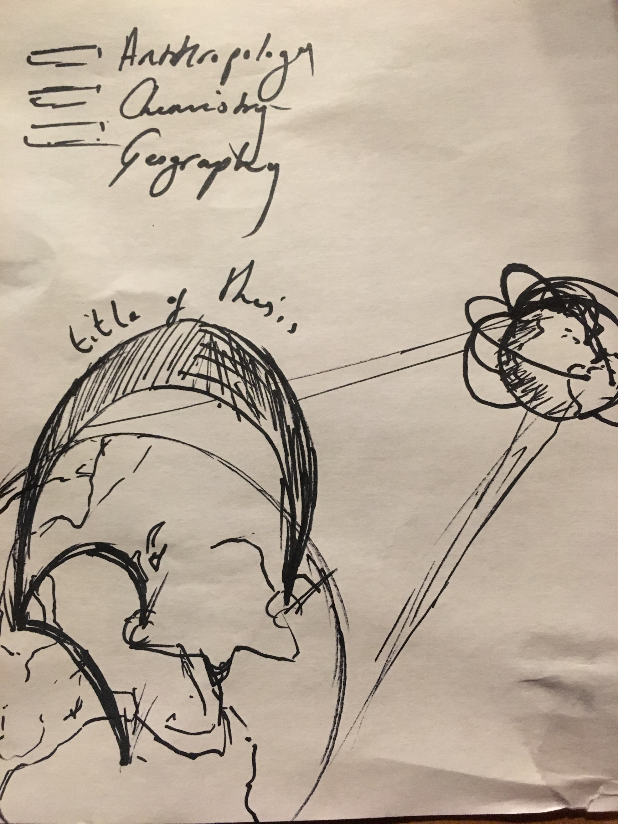
Preliminary sketches
The prevalence of globalisation has enabled researchers from all departments travel the world with great ease and share their findings within the university domain. For my final project, I want simultaneously display the geographic reach of departmental research published at UCSB, and develop a tool for the general public to interrogate Santa Barbara’s connection to other locations across the world.
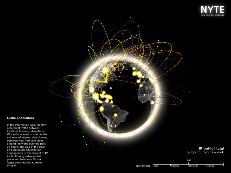
My strategy is inspired by the metaphor of global networks attributing cultures traditions and histories to different locales, and how researchers travel to investigate these cultural geographies and transfer those resources and knowledge to Santa Barbara. I aim to represent these flows of information from locations to UCSB within my visualisation.
Process
For this assignment I am using the Alexandra Digital Research Library data. I scraped the ADRL UCSB Electronic Theses and Dissertations. To identify any locations specific to the thesis or dissertation I pushed the results through a geoparser which compared the word strings to individual place names in Gazeteers. The geoparsed results were read into R and geocoded using the following code which returns the latitude and longitude of the placename.
I scraped the ADRL UCSB Electronic Theses and Dissertations (N=1731) for the corresponding fields; Title, Year, Author, Degree Grantor, Supervisor, Description, Language, and wrote to csv. To select and group by department I ran the following query.
To identify any locations specific to the thesis or dissertation I pushed the results through a geoparser which compared the word strings to individual place names in Gazeteers. To do this I selected gazeteers at multiple levels of geography and parsed the strings through each, to extract place names from multiple place scales. The gazetteers downloaded were (GeoNames, ADL Gazetteer, U.S. Census, Wikipedia) to cover the potential range of current, historic and informal place names which may be included in the research titles and abstracts.
The geoparsed results are as follows:
- California cities where population > 50,000 as of 2004
o 170 cities: 98/1730 matches
- California cities (all) as of 2010
o 482 cities: 134/1730 matches
- California counties (all)
o 57 counties: 131/1730 matches
- CA urban areas (all)
o 155 urban areas: 99/1730 matches
- U.S. cities (major by population, 2014)
o 297 cities: 128/1730 matches
- U.S. places (Census)
o 29,576 places: 1298/1730 matches
- U.S. counties (Census)
o 3,219 counties: 12/1730 matches
- U.S. urban areas (Census)
o 3,600 urban areas: 595/1730 matches
- U.S. states
o 50 states: 176/1730 matches (cleaned to 166)
- Largest world cities
o 237 cities: 261/1730 matches
- Country names
o 203 countries: 277/1730 matches
This method underperformed in some categories, and because of this I tried implementing a machine learning algorithm Stanford’s Name Entity Recognition, which identifies places, organisations and names within text strings. The output was too difficult to clean in a short space of time so I kept this methodology.
The geoparsed results were read into R and geocoded using code which returns the latitude and longitude of the placename. This data now has the correct information to geographically locate all the thesis and dissertations on to locations on earth.
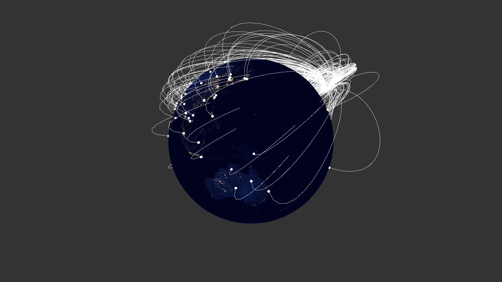
Final result
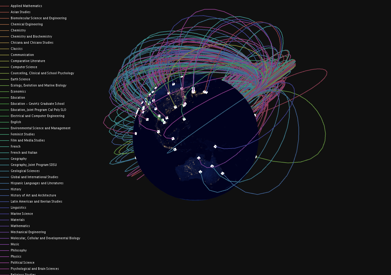
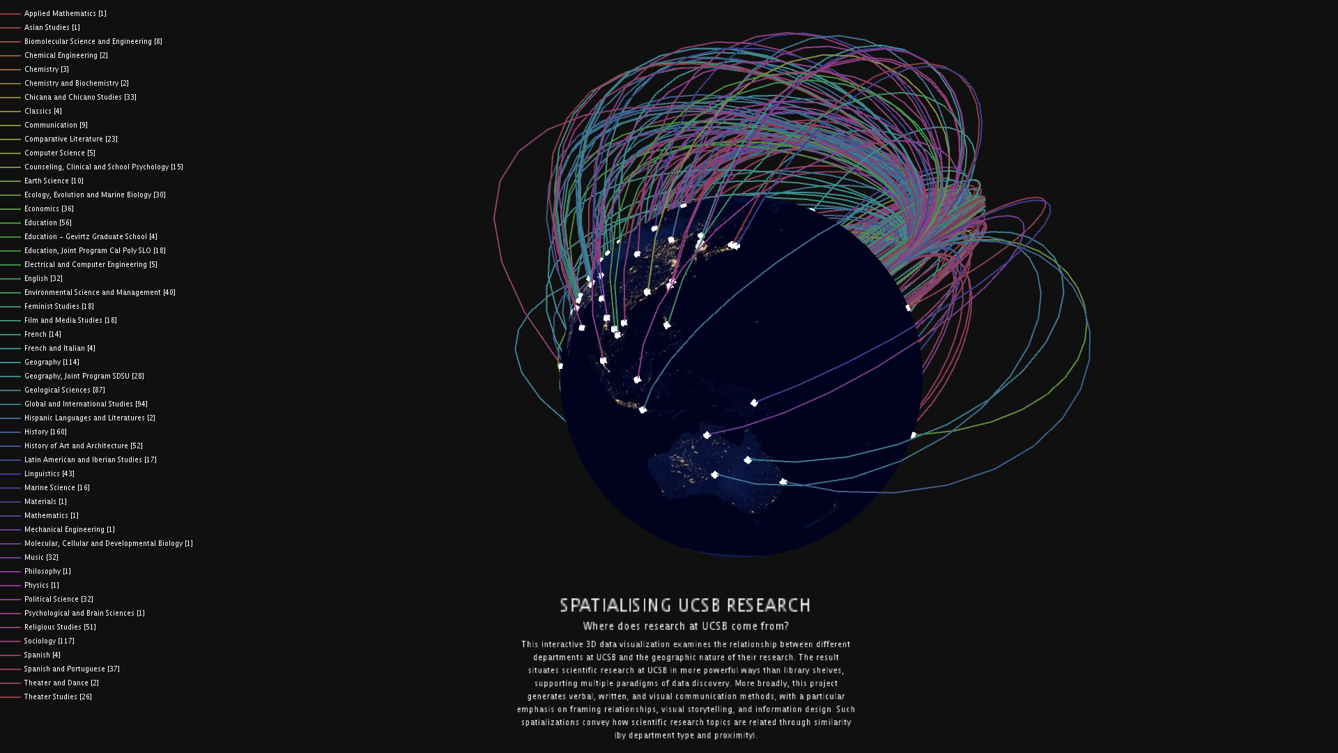
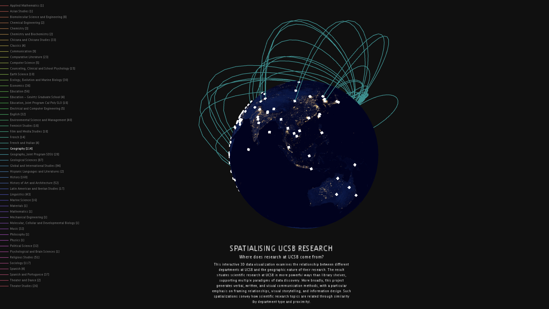
This interactive 3D data visualization examines the relationship between different departments at UCSB and the geographic nature of their research. The result situates scientific research at UCSB in more powerful ways than library shelves, supporting multiple paradigms of data discovery. More broadly, this project allows me to generate verbal, written, and visual communication methods, with a particular emphasis on framing relationships, visual storytelling, and information design. Such spatializations will convey how scientific research topics are related through similarity (by department type and proximity).
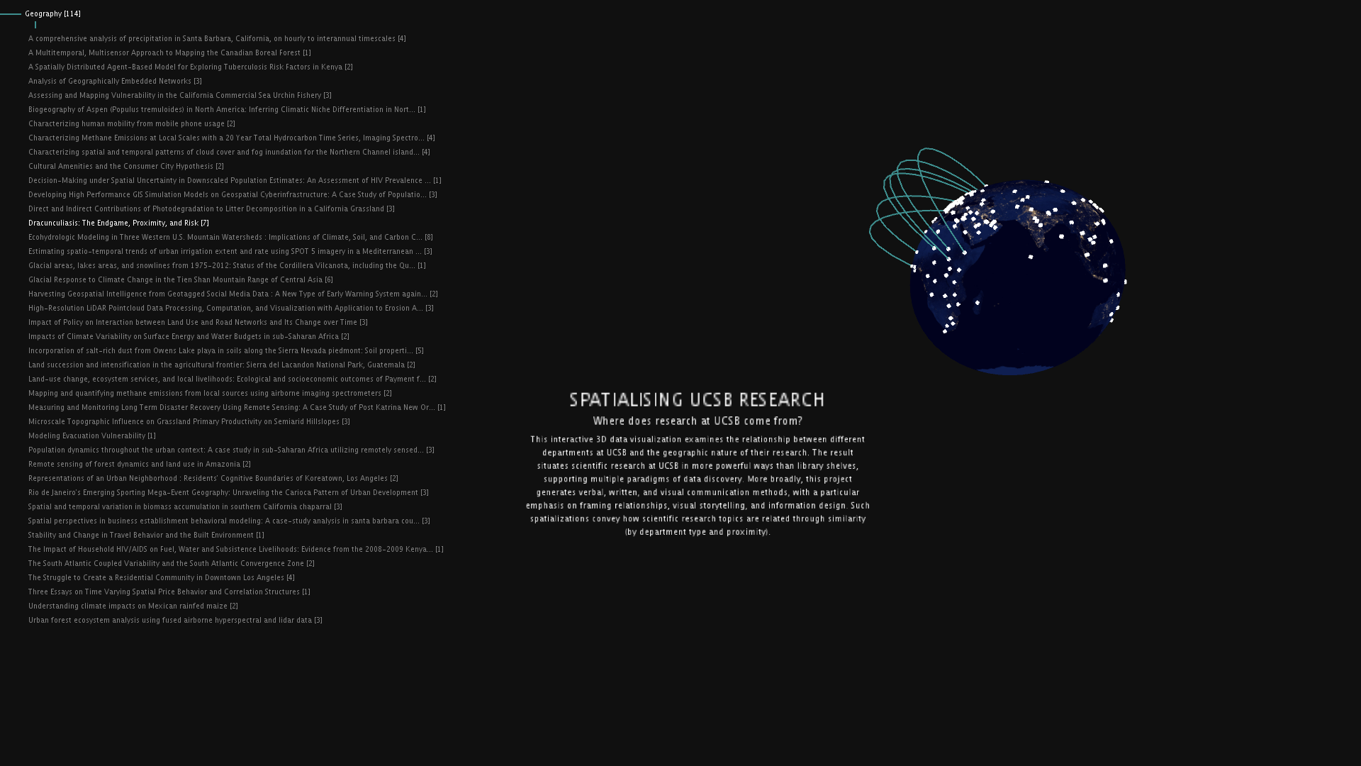
Interactivity was introduced into this model, and each time a department is hovered over in the legend, only those links from that department are shown. This helps the user identify which departments are more ‘spatialised’ than others. As well as this, when the user has selected the department, the titles of the theses or dissertations associated with the geographic placements will be shown. Each of these items has a number in parenthesise provided, which reflects the number of places associated with that department or that thesis. As evident in the visualisation, some theses cover more than one location, which makes for rich geographical history of research at UCSB.
Code