Self-Organizing Map of Checkout Trends
MAT 259, 2015
Donghao Ren
Concept
This project uses Self-Organizing Map and Restricted Boltzmann Machine to visualize temporal checkout trends of each 2nd-level Dewey class in the Seattle Library Dataset.
Query
Query 1 - Extract temporal features:
SELECT
 COUNT(*) AS count,
 TIMESTAMPDIFF(DAY, "2010-01-01 00:00:00", checkOut) AS day,
 deweyClass AS deweyClass
FROM
 transactions,
 deweyClass
WHERE
 transactions.bibNumber = deweyClass.bibNumber
 AND YEAR(checkOut) >= 2010 AND YEAR(checkOut) <= 2014
 AND deweyClass != ""
GROUP BY
 day, deweyClass
Query 2 - Count number of bibs in each Dewey class:
SELECT
 COUNT(*) AS count,
 FLOOR(deweyClass / 10) AS deweyClass2
FROM deweyClass
WHERE deweyClass != ""
GROUP BY deweyClass2
Process
The query extracts the number of checkouts for each Dewey category from 2010 to 2014 monthly. There are 100 Dewey classes and 60 months in total. Each category is represented by its number of checkouts for each month, which form a 60-dimensional vector. We have 100 such vectors, one for each category.
The visualization uses two methods: SOM and RBM+PCA to visualization the temporal trends among these categories. The main goal is to compare the two methods, and see if we can find something meaningful from the visualizations.
The SOM works by taking each Dewey category's trend as an training vector, and then run the SOM for each category to find the winning neuron where the category is drawn at.
The RBM+PCA takes a different approach, which it builds a model by concatenating a RBM and a PCA. Then uses the trends for the 100 categories as training vectors, and finally run the trained model to find the coordinates for each category.
The third view at the bottom is just the trends themselves. A simple hover-and-highlight interaction is implemented.
Final result
Below is my final visualization. Colors show the dewey categories. Left is the SOM map, and right is the RBM+PCA map.
Users can hover on the dewey categories and highlight them in other charts.
By looking at the visualization, we can find that the two maps have some common structures. Some categories that are close to each other in one map can also be close in the other. But there are also counter-examples.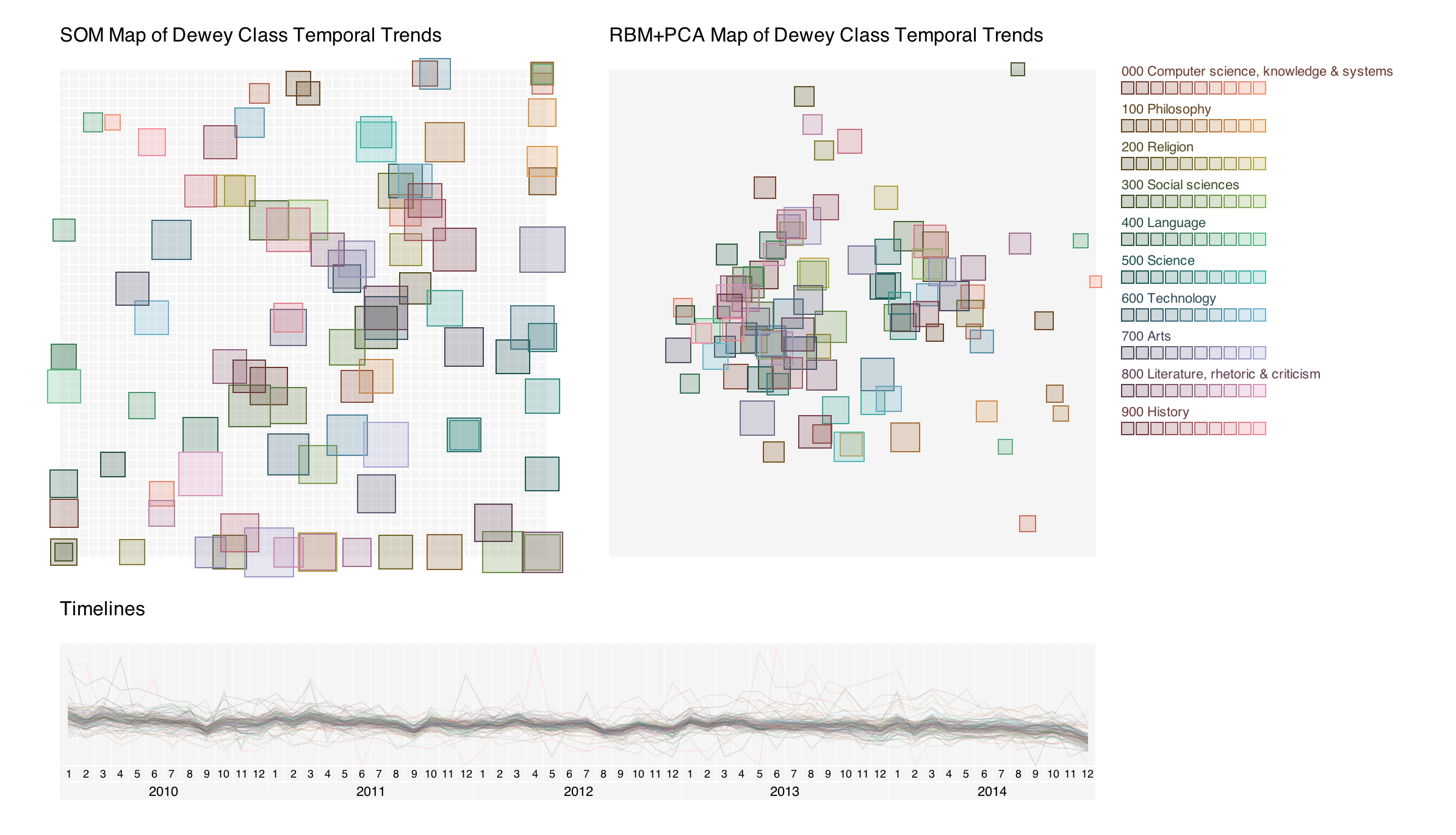
By looking at the visualization, we can find that the two maps have some common structures. Some categories that are close to each other in one map can also be close in the other. But there are also counter-examples.
Code