Skyscrapers: Three-Dimensional Interactive Project
MAT 259, 2013
Jay Byungkyu Kang
Introduction
As the impact of social media such as Facebook or Twitter grows on our daily life, they are considered as crucial tools for various objectives. For instance, most of the major companies use them to develop aggressive marketing strategies. Moreover, recently, Twitter has been widely used as a tactical medium for political campaigns in many countries.
Therefore, I would like to visualize its transition along the timeline in terms of the distribution of transactions of item checkouts which contain names of most frequently used social media (Twitter, Facebook and LinkedIn) in titles. Each of the above social networking services has a distinctive character of its own. In this 3D project, the visualization is based on the checkout history between 2009 - 2012, the heyday of major microblogging services.
Therefore, I would like to visualize its transition along the timeline in terms of the distribution of transactions of item checkouts which contain names of most frequently used social media (Twitter, Facebook and LinkedIn) in titles. Each of the above social networking services has a distinctive character of its own. In this 3D project, the visualization is based on the checkout history between 2009 - 2012, the heyday of major microblogging services.
Background and Sketches
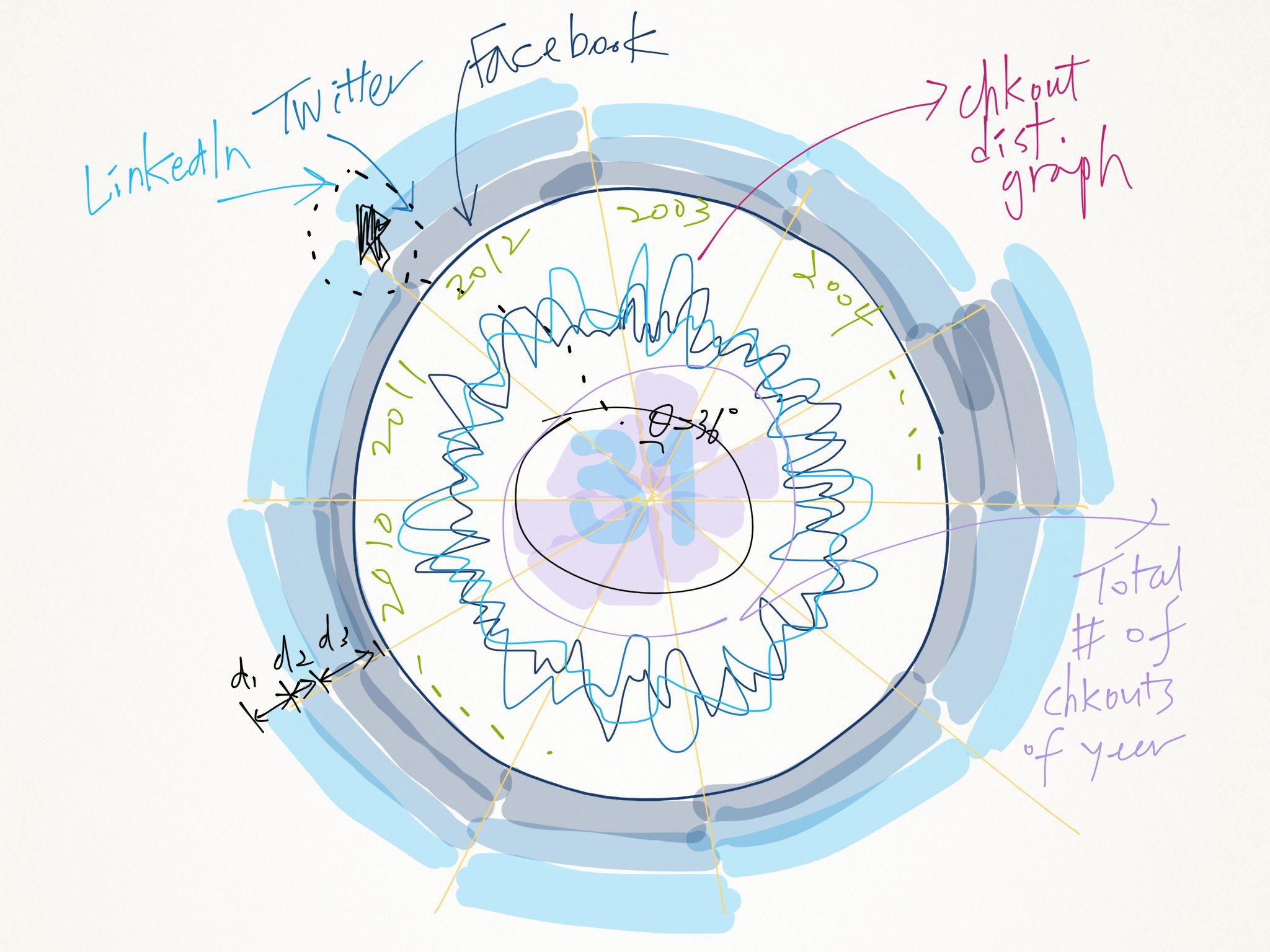
(1) Previous doodle for 2D visualization
The 3D visualization project is intended as an extended version in the 3D space of the previous 2D project. Therefore, I decided to develop the sketch based on the previous doodle for the 2D Viz project. The original doodle is built on a symmetric disk that shows the histogram of checkout history across three different data sets.
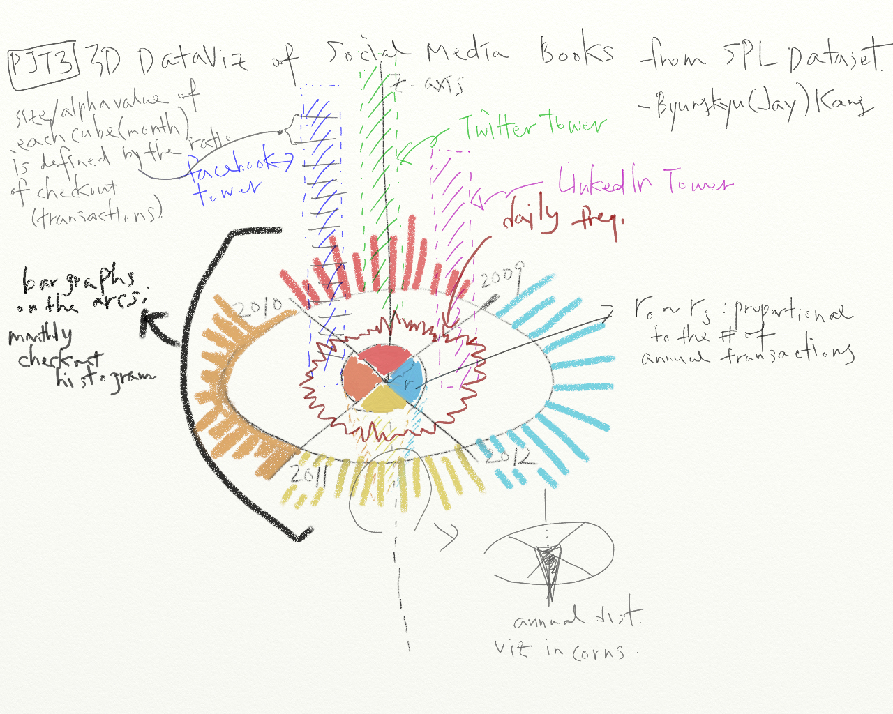
(2) Doodle for 3D visualization
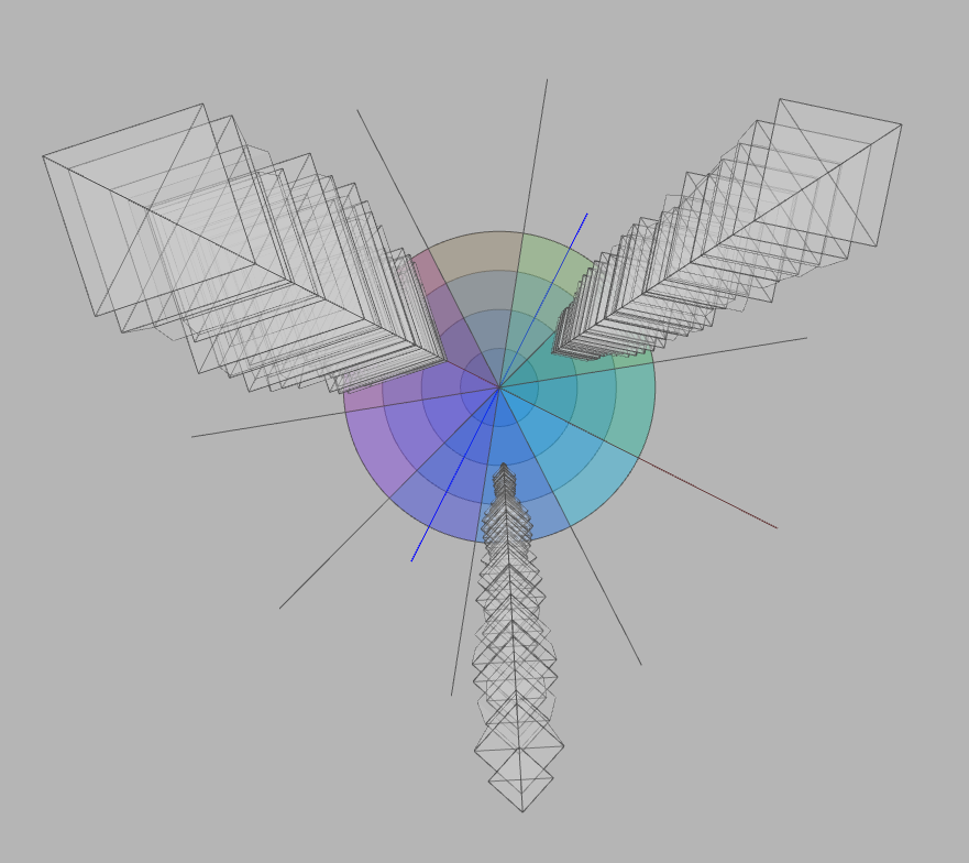
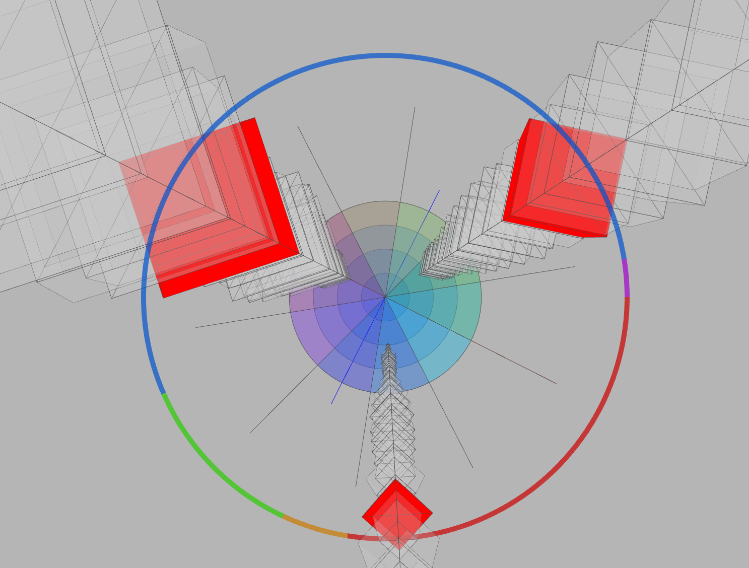
As can be seen in this doodle, I designed to show the histogram of checkouts in the form of a series of cubes stacked on the disk in 3D space. Each cube represents a unit time (each month) with different color intensity or transparency. On the disk, each bar on the rim of the circle represents the sum of transactions of the three data sets in each month.
The 3D visualization project is intended as an extended version in the 3D space of the previous 2D project. Therefore, I decided to develop the sketch based on the previous doodle for the 2D Viz project. The original doodle is built on a symmetric disk that shows the histogram of checkout history across three different data sets.
(2) Doodle for 3D visualization
As can be seen in this doodle, I designed to show the histogram of checkouts in the form of a series of cubes stacked on the disk in 3D space. Each cube represents a unit time (each month) with different color intensity or transparency. On the disk, each bar on the rim of the circle represents the sum of transactions of the three data sets in each month.
Query
This query is run on the ‘spl1’ database computing distribution of transactions across different keywords in title and different dewey categories between 2009 and 2012.
int[] keywords = {‘facebook’, ‘twitter’, ‘linkedin’};
for each:
"SUM(CASE WHEN dewey.dewey BETWEEN 0 AND 99 THEN 1 ELSE 0 END) as d0," + "SUM(CASE WHEN dewey.dewey BETWEEN 100 AND 199 THEN 1 ELSE 0 END) as d1," + "SUM(CASE WHEN dewey.dewey BETWEEN 200 AND 299 THEN 1 ELSE 0 END) as d2," + "SUM(CASE WHEN dewey.dewey BETWEEN 300 AND 399 THEN 1 ELSE 0 END) as d3," + "SUM(CASE WHEN dewey.dewey BETWEEN 400 AND 499 THEN 1 ELSE 0 END) as d4," + "SUM(CASE WHEN dewey.dewey BETWEEN 500 AND 599 THEN 1 ELSE 0 END) as d5," + "SUM(CASE WHEN dewey.dewey BETWEEN 600 AND 699 THEN 1 ELSE 0 END) as d6," + "SUM(CASE WHEN dewey.dewey BETWEEN 700 AND 799 THEN 1 ELSE 0 END) as d7," + "SUM(CASE WHEN dewey.dewey BETWEEN 800 AND 899 THEN 1 ELSE 0 END) as d8," + "SUM(CASE WHEN dewey.dewey BETWEEN 900 AND 999 THEN 1 ELSE 0 END) as d9," + "count(*), DATE_FORMAT(o,'%Y-%m') as coutmonth " + "FROM title, activity, dewey " + "WHERE title.bib = activity.bib AND activity.bib = dewey.bib AND LOWER(title) like '%" + keywords[kw] + "%' AND year(o) > 2008 AND year(o) < 2013 GROUP BY coutmonth;";
Process
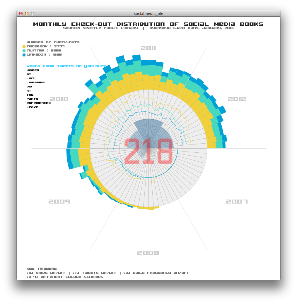
2D Version:
As can be seen below, we can easily see the transition of popularity of social media implied in the form of the distribution of the checkouts of relevant materials in the Seattle Public Library. We can also compare the popularity(in the number of transactions) across different years or months. Moreover, the implementation is delivering some interactivity. For example, you can enable or disable a few functionalities such as grids, daily frequency distribution, total number of checkouts of each month by using trigger keys or hovering the mouse cursor on each bar.
This description is provided for comparison with 3D visualization.
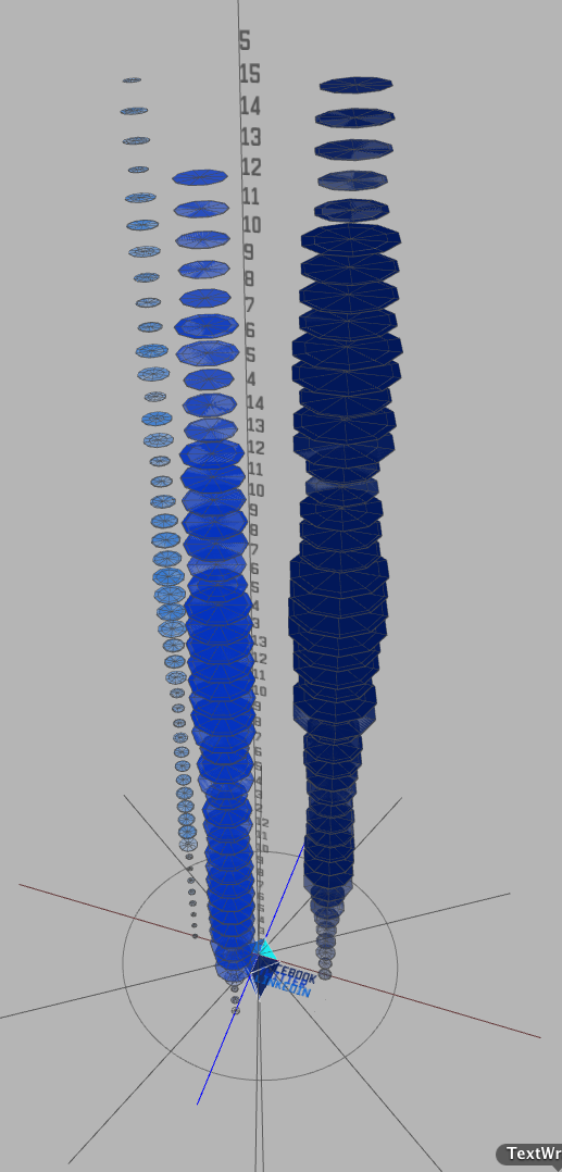
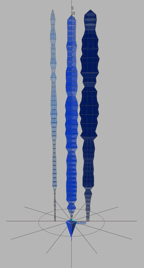
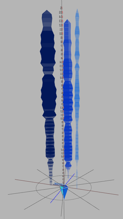
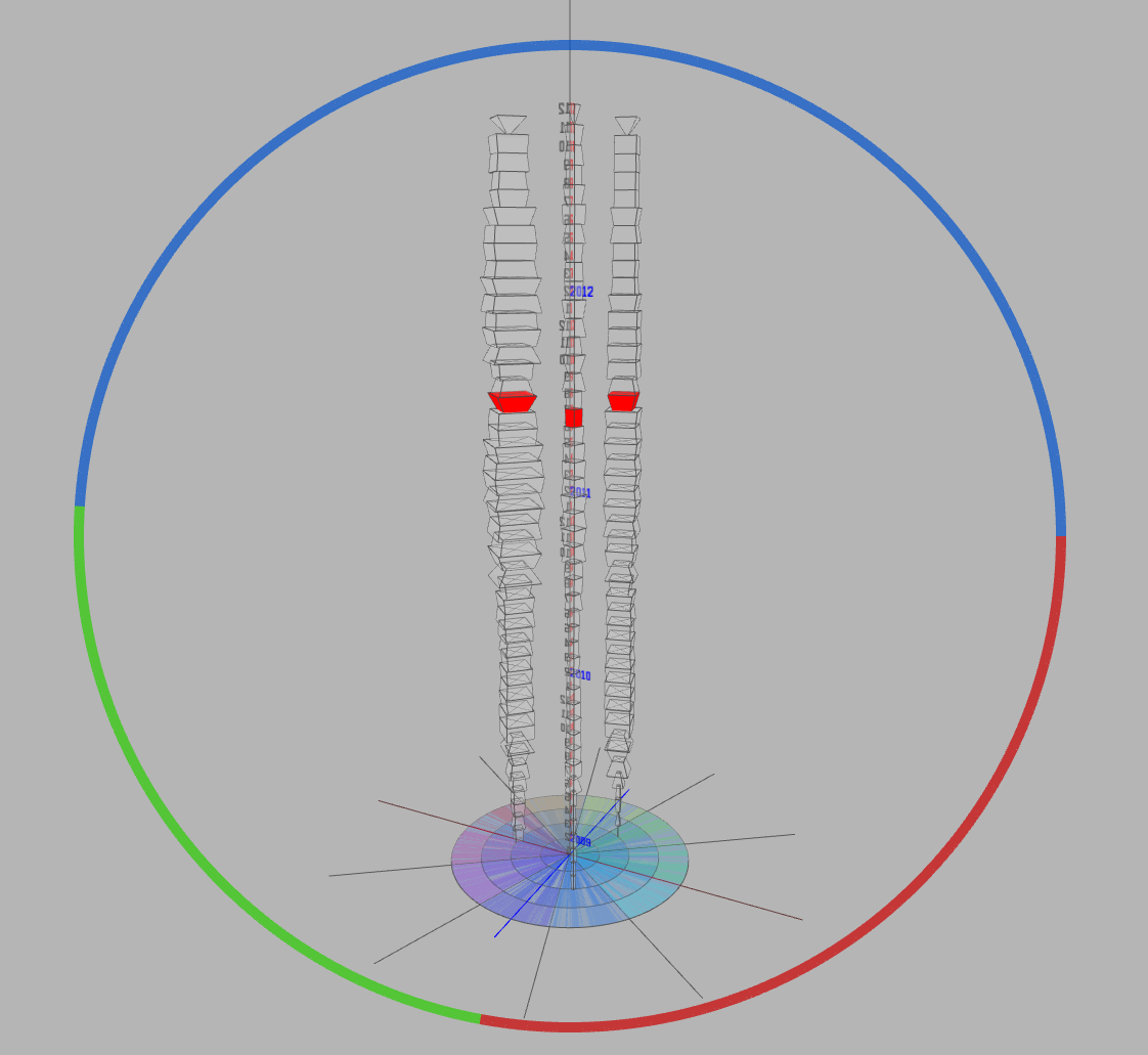
Using the above query, I was able to fetch each data set upon corresponding keyword (‘facebook’, ‘twitter’ and ‘linkedin’) from MYSQL database. The ‘spl1’ database, which has been modularized and indexed for the sake of performance, was chosen. Afterwards, I tried to visualize this time-variant data along the z-axis. In order for users of this application easily comprehend the transition of each data, I decided to change each cube with different dimension based on corresponding item checkout number. (a) The visualization below used a cylinder structure with 10 sides.
As can be seen below, we can easily see the transition of popularity of social media implied in the form of the distribution of the checkouts of relevant materials in the Seattle Public Library. We can also compare the popularity(in the number of transactions) across different years or months. Moreover, the implementation is delivering some interactivity. For example, you can enable or disable a few functionalities such as grids, daily frequency distribution, total number of checkouts of each month by using trigger keys or hovering the mouse cursor on each bar.
This description is provided for comparison with 3D visualization.
Using the above query, I was able to fetch each data set upon corresponding keyword (‘facebook’, ‘twitter’ and ‘linkedin’) from MYSQL database. The ‘spl1’ database, which has been modularized and indexed for the sake of performance, was chosen. Afterwards, I tried to visualize this time-variant data along the z-axis. In order for users of this application easily comprehend the transition of each data, I decided to change each cube with different dimension based on corresponding item checkout number. (a) The visualization below used a cylinder structure with 10 sides.
Results and Analysis
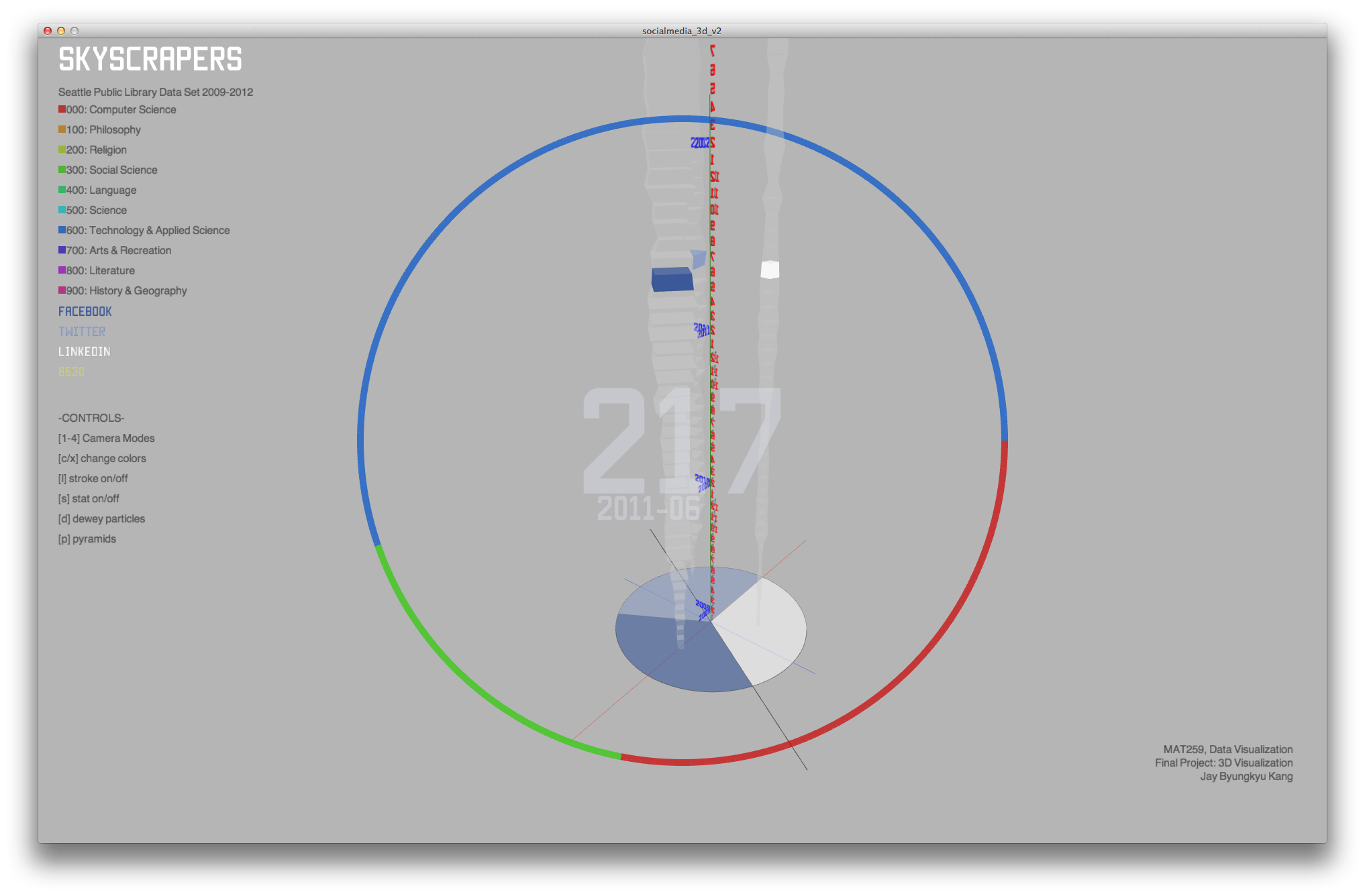
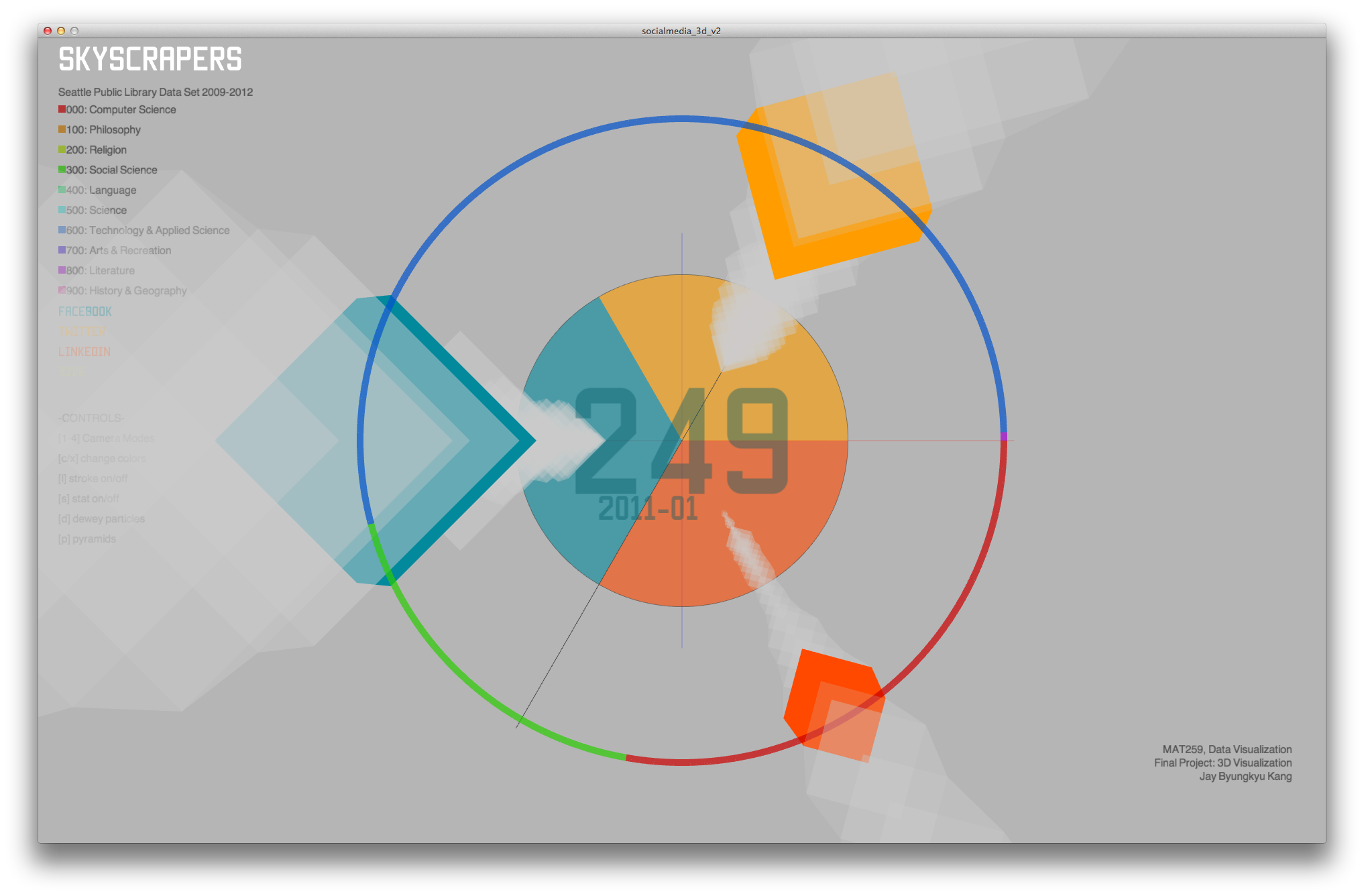
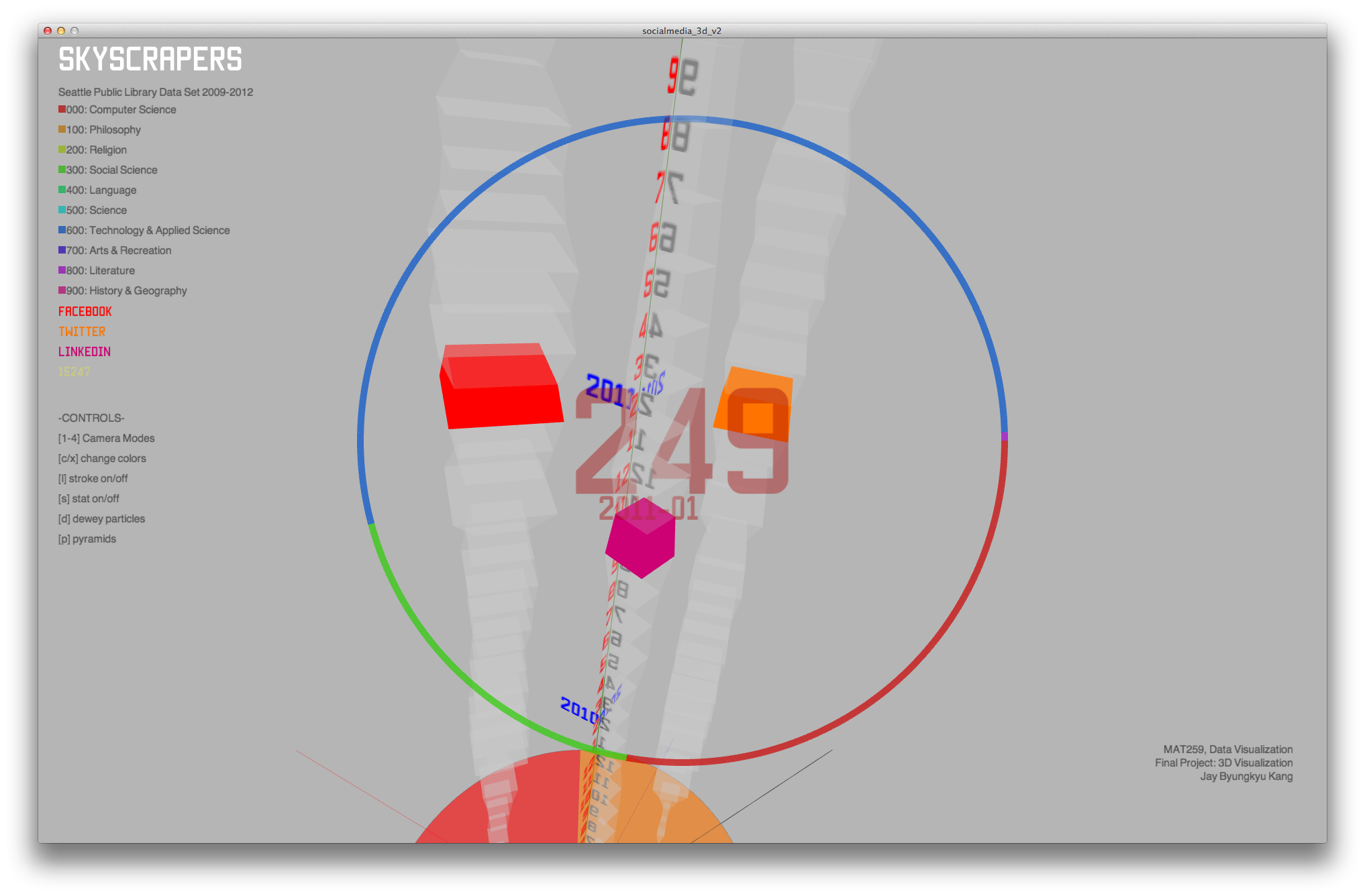
(g) Final visualization with labels, legends and optimized color schemes.
Code
I used Processing and Peasycam.
A function called ‘drawCylinder’ is used. This function is taken from the book: ‘Processing: a programming handbook for visual designers and artists’ written by Casey Reas and Ben Fry.
Run in Browser
Source Code
A function called ‘drawCylinder’ is used. This function is taken from the book: ‘Processing: a programming handbook for visual designers and artists’ written by Casey Reas and Ben Fry.
Run in Browser
Source Code
Control
Press 1-4 for different camera views
c/x : change to different palette (0 to 10)
l : stroke on / off
s : Stat view on / off
d : dewey particles
p : pyramids on / off (checkouts in each year below the disk)
5: FP-Tree 2
6: Pyramids
7: Side view
8: Random view
9: Toggle rotation
Control Parameters
G: Hide/Show Grid
L: Hide/Show Lines
P: Hide/Show Pyramids
V: Toggle Variance
Parameters
Master Rotation
Node Spacing
Root Distance
Branch Spread
Rotation Speed